FPGA-Signalverarbeitungs-Pipeline: FIR, FFT und DDS in Logik aufbauen
FPGA signal processing is fundamentally different from CPU work — a CPU runs one instruction per sample, while an FPGA produces one result per clock cycle. How to build FIR without stalling the pipeline, how many FFT points you actually need, and how to configure the DDS phase accumulator — this article walks through the RTL implementation and resource budget for three core modules.
1. Why FPGA Is Built for Real-Time Signal Processing
CPU/DSP processes signals serially: one multiply-add per clock, then moves to the next sample. FPGA is a parallel pipeline: multipliers, adders, and registers are fully unrolled, outputting one result every clock cycle.
| Metric | CPU (single core) | FPGA |
|---|---|---|
| Single-channel FIR throughput | MSa/s range | GS/s range |
| Multi-channel parallel | Needs multi-core/multi-chip | Unroll N channels on one chip |
| Latency | Milliseconds (OS scheduling) | Nanoseconds (deterministic) |
| Dynamic reconfiguration | Recompile software | Recompile hardware |
Core advantage: FPGA latency is deterministic — N pipeline stages means exactly N clock cycles, unaffected by OS, cache, or interrupts. This is a hard requirement for radar, SDR, and industrial control where the next sample must be processed before it arrives.
2. FIR Filter: Build It Without Stalling the Pipeline
FIR is mathematically simple: y[n] = Σ(h[k] × x[n-k]), a sum of multiply-accumulates across taps. But how you implement it in FPGA logic directly affects resource use and timing closure.
2.1 Direct Form vs Transposed Form
| Structure | Multiplier placement | Latency | Best for |
|---|---|---|---|
| Direct form | One multiplier per tap, add stage by stage | N cycles | Few taps (< 32) |
| Transposed form | Parallel multipliers, results feed an adder tree | log2(N) cycles | Many taps (64+), better timing |
Practical advice: use direct form for ≤ 32 taps, transposed form for ≥ 64 taps. Transposed form uses more adders but has registers after each multiplier, shortening the critical path and making 300+ MHz easier.
2.2 Bit Width Selection
14-bit ADC input, 16-bit coefficients → 30-bit product. Outputting 30 bits directly breaks the next FFT stage, so truncation is required.
- Accumulator width: keep full precision (30 bits is enough, don’t truncate early)
- Output truncation: based on SNR requirements. 14-bit ADC gives ~86 dB SNR; keeping 18–20 bits at FIR output is sufficient
- Where to truncate: at the end of the adder tree, not at each stage (accumulating quantization noise)
2.3 Resource Estimate (XCKU15P example)
A 64-tap, 14-bit input, 16-bit coefficient FIR:
| Resource | Usage | XCKU15P total | Utilization |
|---|---|---|---|
| DSP48E2 | 64 | 1,968 | 3.2% |
| BRAM | ~0 | 744 | — |
| LUT | ~2,000 | 130,000 | 1.5% |
A 64-tap FIR uses only 3% of DSPs on UltraScale. Eight parallel channels multiply that by 8, still only 25%.
3. FFT: How Many Points, Which IP, How Much Latency
FFT is the most common frequency-domain analysis tool. Choosing between 1024 and 4096 points, radix-2 vs radix-4, and measuring pipeline latency directly determines whether real-time operation is feasible.
3.1 Point Count Selection
| FFT points | Frequency resolution (100 MHz sample) | Time window | Best for |
|---|---|---|---|
| 256 | 390 kHz | 2.56 µs | Fast spectrum monitoring |
| 1024 | 97.7 kHz | 10.24 µs | General spectrum analysis |
| 4096 | 24.4 kHz | 40.96 µs | Fine spectrum / frequency measurement |
| 16384 | 6.1 kHz | 164 µs | Narrowband signal measurement |
Trade-off: more FFT points means better frequency resolution, but longer time windows. For frequency-hopping signals (e.g. radar pulses), a long window averages across hops and blurs the picture.
3.2 Pipelined vs Burst I/O
Xilinx FFT IP offers two architectures:
| Architecture | Throughput | Latency | Resources | Best for |
|---|---|---|---|---|
| Pipelined | 1 sample per clock | ~N/2 cycles | Large | Real-time continuous data |
| Burst I/O | N samples per batch | Wait for batch | Small | Non-real-time / offline |
Real-time systems must use Pipelined. Burst I/O saves resources but has gaps between batches, unsuitable for continuous sample streams.
3.3 Latency Calculation
For 1024-point Pipelined FFT at 250 MHz:
- Data throughput: 250 MSa/s
- Frame latency: 1024 / 250M = 4.096 µs (from input done to output)
- Plus ~30% internal FFT core overhead, total ~5.3 µs
If your system requires results within 10 µs of sampling, 1024-point FFT works. For 4096 points, latency rises to ~21 µs and may not meet the spec.
4. DDS: How to Configure the Phase Accumulator
DDS (Direct Digital Synthesis) generates sine/cosine local oscillator signals for SDR, radar, and communications.
4.1 Basic Principle
DDS is a phase accumulator plus lookup table:
- Phase increment M determines output frequency
- f_out = M × f_clk / 2^N (N = phase bit width)
| Parameter | Typical value | Notes |
|---|---|---|
| Clock f_clk | 250 MHz | Sampling clock |
| Phase width N | 26–32 bit | Determines frequency resolution |
| Table width | 16–18 bit | Determines SFDR |
| Output freq | ≤ f_clk / 2 | Nyquist limit |
Example: 250 MHz clock, 32-bit phase accumulator, 70 MHz LO output:
- M = 70M × 2^32 / 250M = 1,202,592,069
- Frequency resolution = 250M / 2^32 ≈ 0.058 Hz
0.058 Hz step is more than enough for SDR local oscillators.
4.2 Resource Usage
A 250 MHz, 16-bit output DDS:
- Block RAM: ~1 block (sine table, 4096 × 16 bit)
- DSP: 0 (lookup + adder, no multiplier needed)
- LUT: ~500
DDS is the lightest signal processing module. Eight parallel DDS channels need only 8 BRAM blocks.
5. Wiring It Together: A Complete Signal Processing Pipeline
Connect FIR → FFT → DDS to form a typical SDR/radar receive chain:
“`
ADC 14 bit
→ FIR lowpass (64 taps, 250 MHz)
→ Downconversion (DDS LO × mixer → lowpass)
→ FFT 1024-point (spectrum analysis)
→ Detect / send to PCIe
“`
Timing budget (250 MHz clock):
| Stage | Latency |
|---|---|
| FIR 64 taps | 64 / 250M = 256 ns |
| DDS mixer | 1 / 250M = 4 ns (1 cycle) |
| FFT 1024-point | ~5.3 µs |
| Total | ~5.6 µs |
4 ns per clock, total pipeline latency 5.6 µs. Compare to CPU FFT in the tens of milliseconds — FPGA is nearly 4 orders of magnitude faster.
6. Board Selection Guidance
| Application | Recommended board | Why |
|---|---|---|
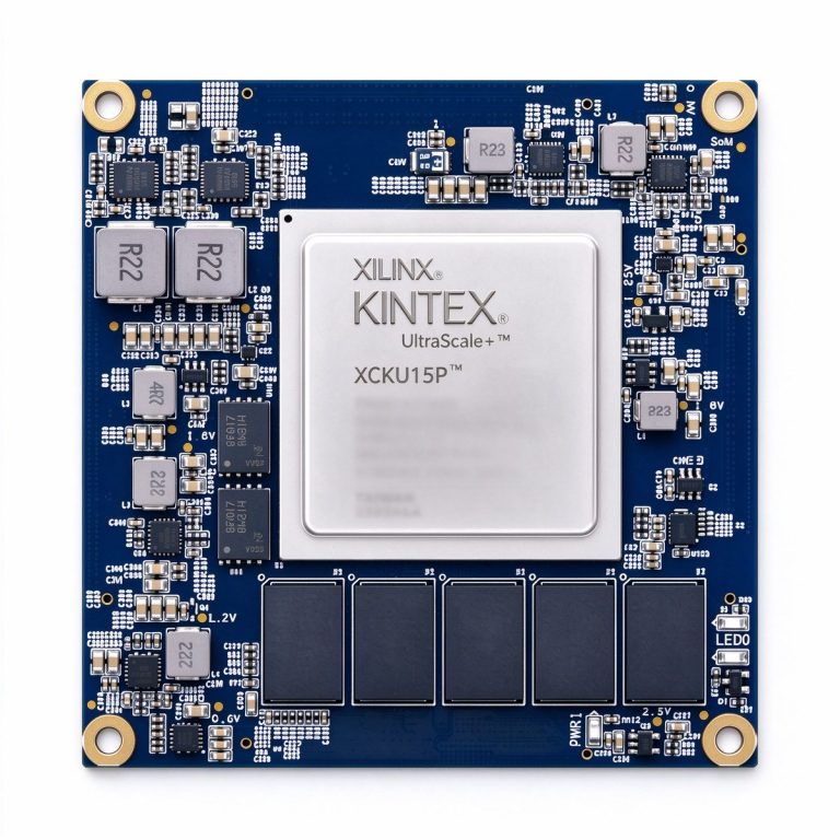
| Radar / phased array / multi-channel acquisition | XCKU15P (Kintex UltraScale) | 1,968 DSPs, 32 GTH transceivers, multi-channel parallel processing |
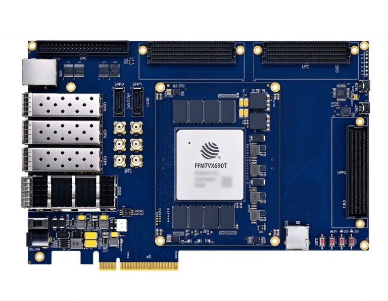
| SDR / JESD204 direct RF sampling | DUF7690T (JFM7VX690T) | Virtex-7 equivalent with ample DSPs, China domestic alternative |
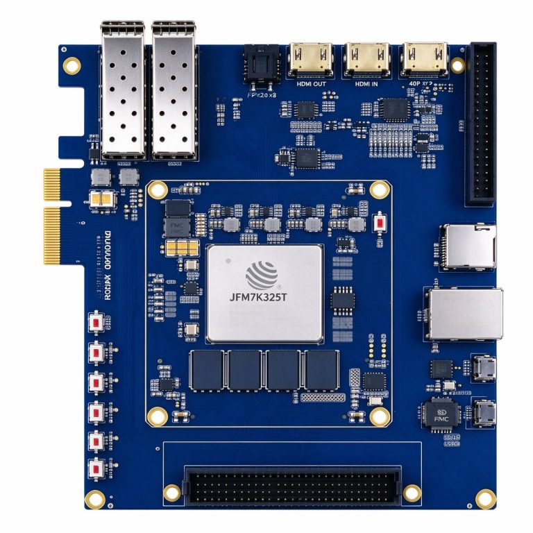
| Mid-speed acquisition / industrial control / cost-sensitive | DUK7325T (JFM7K325T) | Kintex-7 class, enough DSP for single-channel FIR+FFT, low cost |
Resource rule: list your channel count × FIR taps × FFT points, then compare against the board’s DSP count. As a rule of thumb, keep DSP utilization under 60% for headroom.
There is no silver bullet in signal processing — direct vs transposed FIR, FFT point count, DDS phase width all depend on your sample rate, latency budget, and resources. Draw the timing budget table first, then pick the board, not the other way around.
Related Products
- DUKU15P (XCKU15P Kintex UltraScale SOM): 1,968 DSP48E2 units for multi-channel radar/SDR processing
- DUF7690T (JFM7VX690T Development Board): Domestic Virtex-7 alternative with JESD204 high-speed ADC direct sampling
- DUK7325T (JFM7K325T Development Board): Kintex-7 class for mid-speed acquisition and industrial control
Further Reading
- [Broadband SDR Frontend: RF to Digital Signal Chain](#)
- [JESD204B/C High-Speed ADC/DAC Interface](#)
- [FPGA Clock Tree and Jitter Budget](#)